Practice Work Session
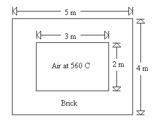
A steady-state heat transfer analysis of a furnace wall shown is shown in the figure below. The air within the furnace is maintained at 560°C. The outside surface of the furnace is exposed to air at 30°C. The furnace wall is made of brick. The problem is to determine the temperature distribution in the brick wall and the total rate of heat transfer through the wall.
By default, FEHT is configured for steady-state heat transfer problems in Cartesian coordinates. These characteristics apply to this practice problem and do not need to be changed.
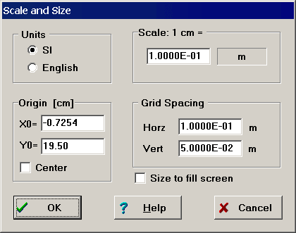
It is usually best to set the unit system, scale, and grid spacing at the start of a problem although they can be changed at any time. Pull down the Setup menu and select the Scale and Size command which will bring up a dialog window in which the scale attributes can be entered.
The small circles in the Scale and Size dialog window shown below are called radio buttons. Radio buttons control the unit system for heat transfer problems. To change the unit system, move the mouse to position the cursor on the appropriate button and click the mouse button. A reasonable scale for this problem is to have 1 cm on the screen represent 0.1 m. Any item within a box can be changed. The unit for length is, by default, centimeters but it can be changed from millimeters to kilometers by clicking in the units box to the right of the scale value. (In the English system, the length unit can be changed from inches to miles.) Click in the scale units box until it displays m for meters. Then enter 0.1 in the scale edit box. Note that double-clicking within any edit box causes the characters to be highlighted (shown in inverse). Typing any character will replace the highlighted field with the entered character. X0 and Y0 designate the location of the origin of the coordinate system on the screen in screen coordinates. The default values, X0=0.0, Y0=0.0 correspond to the origin being placed at the lower left of the screen. Gridlines make the drawing easier to prepare. Grid spacing is specified in the same coordinates as for the drawing. Set the grid spacing as shown below. Click the OK button or press the Enter key to set these scale attributes.
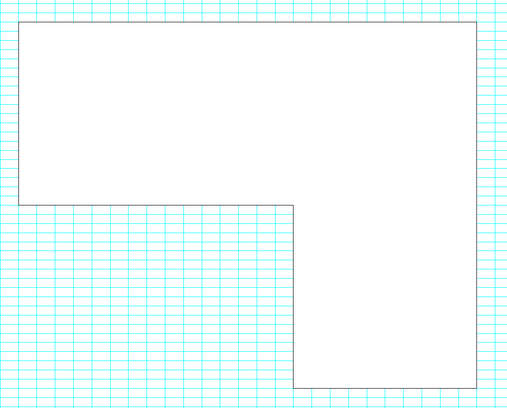
The first step is to sketch material outlines. It is easier to prepare a scale drawing with a coordinate grid. Select Show Grid from the Display menu. Select Outline from the Draw menu. Since this problem is symmetrical, we only need to analyze one quarter of the furnace. Note that the X and Y coordinates of the cursor position for the selected unit system and scale are shown in the small window at the upper left, just below the menu bar. Move the mouse to locate the cursor at position X=0.50 m, Y=2.50 m . Click the mouse to fix a node at the corner. The first node is shown as a small closed circle. Now, position the cursor at X=3.00 m, Y=2.50 m and click the mouse. Hold the shift key down to provide a drawing aid for horizontal, vertical, or 45 degree lines. Click on the remaining corners at X=3.00 m, Y=0.50 m; X=2.00 m, Y=0.50 m; X=2.00 m, Y=1.50 m; and X=0.50 m, Y=1.50 m. Now click on the first corner. The outline must begin and end on the same node without crossing any existing lines. At this point, the outline will flash, indicating that the outlining process is completed and the material within the flashing boundary is selected.
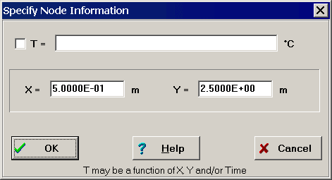
At this point, you may wish to exactly locate the node positions since it unlikely that you were able to do so while drawing with the mouse. Click on the node at the upper left of the drawing and then select the Boundary Conditions command in the Specify menu. (Note that, as a short cut, you can accomplish the same result by double-clicking the mouse on the node.) The Specify Node Temperature dialog window will appear with edit boxes for the node temperature and for the X and Y coordinates of the node. In this case, we wish to alter the coordinates, not the node temperature. Enter the coordinates X=0.50 and Y=2.50 as shown below. FEHT will not let the node move to a position which causes existing lines to cross, so there is some restriction on the coordinates that you enter. Repeat this process for all of the other nodes so that they are exactly positioned at the proper locations. After entering the coordinates of all of the nodes, save the file as Example 1.fet using the Save command in the File menu.
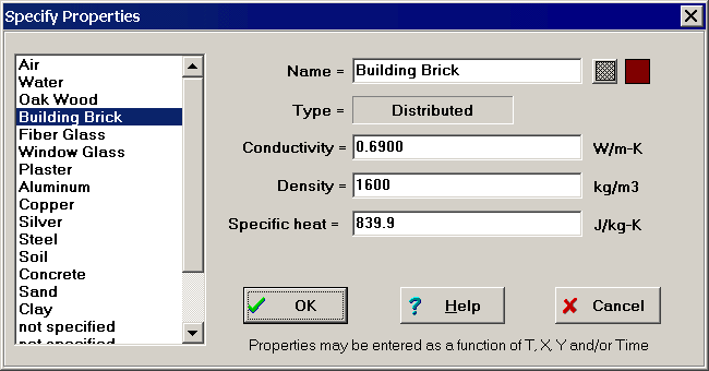
A material must be selected (flashing) in order to specify its properties. A material can be selected by clicking the mouse anywhere within it outline; it is automatically selected just after it has been drawn. Select Material Properties from the Specify menu. A property dialog box will appear with default property names listed on the left. Choose the material to be brick by clicking on Building Brick in the list on the left. You can choose the pattern which will be used to identify the material by holding the mouse button down while the cursor is in the pattern box. A pop-up palette will appear with the possible patterns. The color of the pattern can also be selected in the same manner by clicking in the Color box. The thermal properties of brick are displayed. These properties can be changed to other values. They may also be entered as a function of temperature and position. Leave the brick properties at their default values. The properties dialog box should now appear like this.
Click the OK button and the screen will be redrawn with the pattern you have chosen identifying the material.
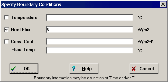
Next we will set the boundary conditions. The vertical line at X=0.50 m and the horizontal line at Y=0.50 m are lines of symmetry and therefore there is zero heat flow across these lines. Move the cursor to a point near the center of one of these lines and click the button. The line should now be flashing. Move the cursor to the center of the other line and click. Both lines should now be flashing. Once a boundary is selected (flashing), the Boundary Conditions menu item in the Specify menu becomes accessible. Select this menu item to bring up the Boundary Conditions dialog window. Enter 0 (for adiabatic conditions) in the Heat Flux box and click the OK button. A check mark will automatically appear in before the word Heat Flux to confirm that you are setting a heat flux boundary condition.
The two boundary lines are now shown with bold lines to indicate that the boundary conditions have been specified.
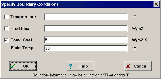
The inside and outside walls of the brick are convective boundaries. Click the mouse at a point near the center of each outside line causing them to flash. Again, select Boundary Conditions from the Specify menu Enter a convection coefficient of 5 W/m2-K and a fluid temperature of 30 C. The dialog window will appear as shown. Click OK.
The convection boundary information for the inside furnace walls is entered in the same manner. Select both boundaries and again issue the Boundary Conditions command. Enter the convection coefficient of 10 W/m2-K and a fluid temperature of 560 C. Click the OK button.
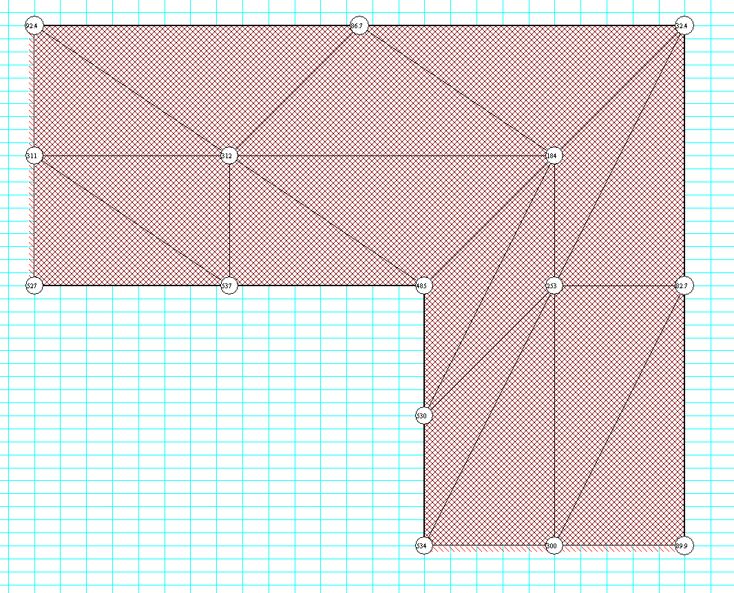
To complete the problem definition, it is necessary to discretize the brick material into triangular elements. This task can be done manually (using the Element Lines command in the Draw menu) or automatically using the Auto Mesh command in the Draw menu. Select the Auto Mesh command. EES will break the outline into triangular elements as shown.
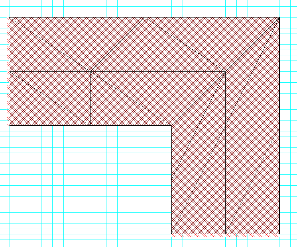
The Auto Mesh command first breaks the outline into a crude mesh and then reduces the mesh once. If you wish to see the crude mesh, select the Undo command. Use the Reduce Mesh command to return to the display above.
Although there it is usually unnecessary, you can adjust the mesh that has been created using the Reposition Nodes command in the Draw menu. You can add additional elements manually to the existing mesh (or create the mesh from the start) by selecting the Element Lines command from the Draw menu. Click on an existing node or line to form one end of the element line. Then click on a node or line that will become the other end of the element line. The following rules apply to manual element line construction.
- The first end of the line must be on an existing line or node. A new node will form at this point if one is not already there.
- Element lines can not cross existing lines.
- Clicking in the area surrounding the drawing or pressing the Esc key cancels the Element Lines command.
The problem definition is complete. Select the Calculate command from the Run menu to initiate the calculations. FEHT will first check the problem definition to ensure that the distributed materials are properly discretized and all properties and boundary conditions are specified. Any errors detected will be listed in the information window at the upper right of the screen, just below the menu bar. This example problem is assumed to be steady-state. Had this been a transient problem (by selecting Transient from the Setup menu), a dialog box would have appeared in which the start, stop and step times would be entered. If no errors are found, a dialog window will appear indicating that the calculations are in progress. When the calculations have been completed, the dialog box will display the elapsed time and other information.
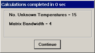
Click the Continue button. A number of the output display windows in the View menu will now be accessible.
The temperatures within the wall can be displayed at each node by selecting Temperatures from the View menu.
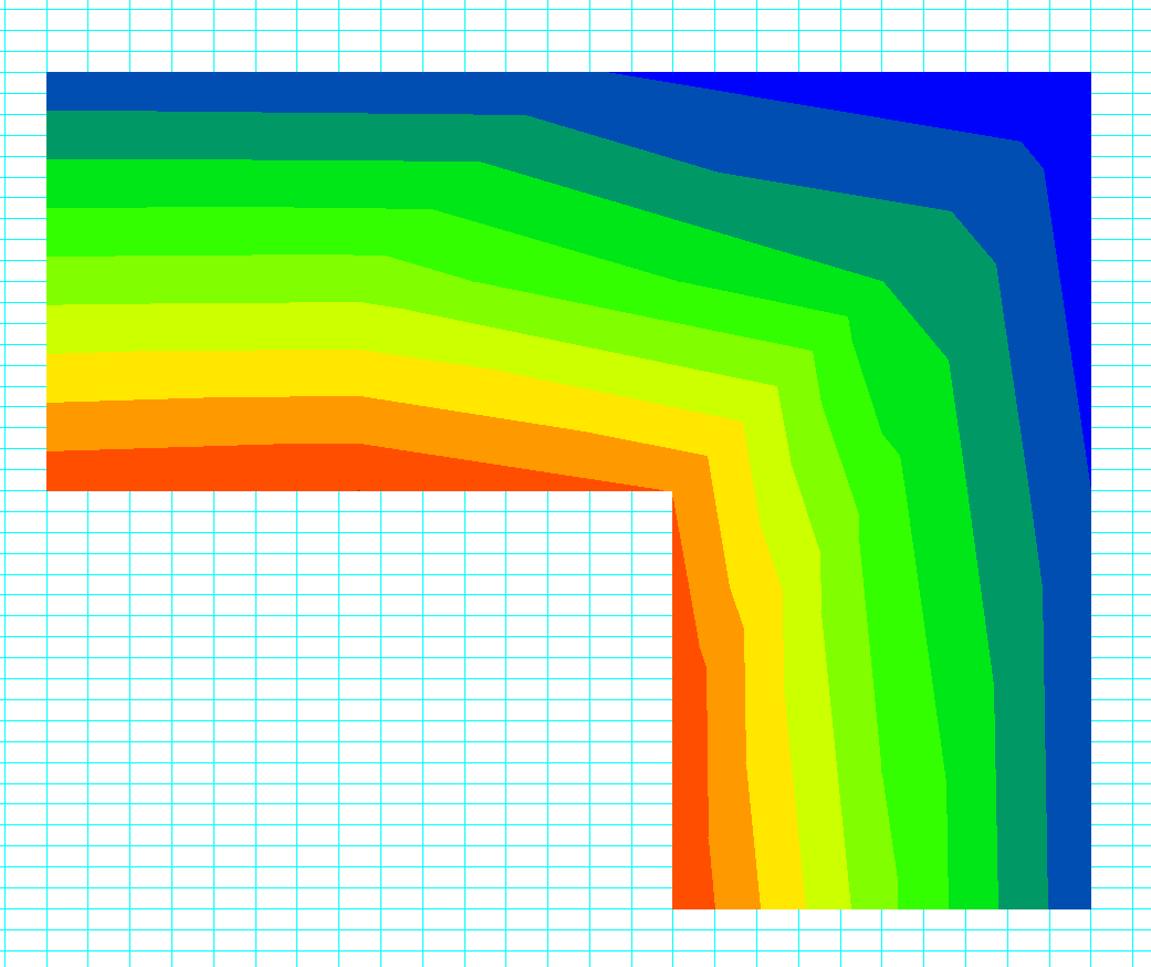
Temperature can also be displayed as a contour plot by selecting Temperature Contours which will bring up the following dialog window.
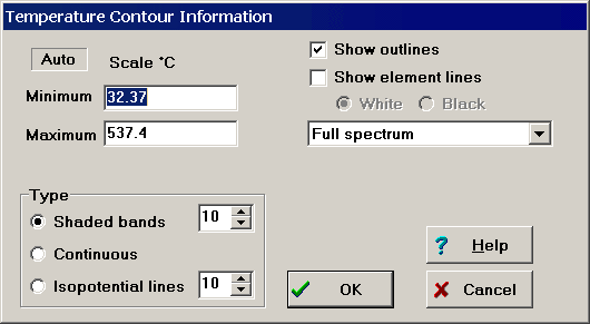
Three types of contour plots are available: continuous colors from red to blud, a banded plot showing gradations of hot to cold (as shown below) and a plot of lines of constant temperatures. The minimum and maximum values in the contour plot can be entered manually or FEHT will automatically find the limits if you click in the User/Auto box at the upper left. Click the OK button or press the enter key to show the contour plot. Note that the contour plot show appears crude because very few nodes were employed. FEHT allows up to 8000 nodes but only 16 were used in this analysis.
In either the temperature or contour plot output, the temperature at the cursor position will be displayed at the upper left of the screen below the menu bar when the mouse button is depressed.
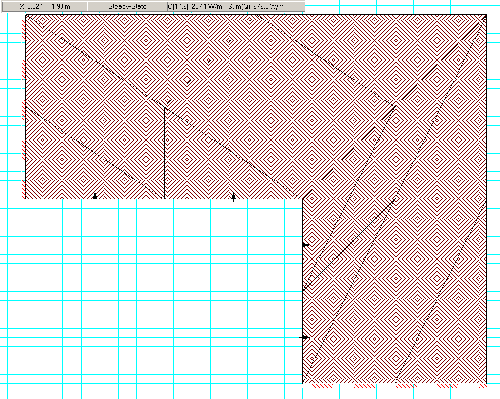
One objective of this problem was to determine the total heat flow through the brick wall. Select Heat Flows from the View menu. (It is also possible to determine the heat flow using the Nodal Balances command, as described in Chapter 2 of the FEHT manual.) The screen will be redrawn with the nodes hidden. Click on any line segment of the inside wall. An arrow will appear indicating the direction of heat flow. The magnitude of the heat flow is shown in the information window at the top right of the screen below the menu bar. Clicking on adjacent lines forming the inside boundary in a clockwise or counterclockwise manner will allow the heat flows to be summed. For one quarter of the problem, the heat flow through the furnace wall is 976.2 W. The total heat flow through all sides of the wall is then 3904.8 W.
Select Input from the View menu to return to the drawing window. At this point, you may wish to explore. Try using smaller triangular elements. FEHT will automatically reduce the mesh size for you if you select the Reduce Mesh Size command in the Draw menu. Will the smaller mesh significantly change the heat transfer rate? How refined does the mesh need to be? Compare the heat flows on the outside walls of the furnace with that on the inside. Should they agree? Do they?