Computational Flow Window
The Computational Flow Window (available in the Professional license) provides information on how EES solves the system of equations in the Main program and Subprograms. It also provides a central point to locate all of the variables defined in the Equations window, Parametric tables, Diagram window, Macros and elsewhere. Included in this window are the blocking and calculation order used by EES, the variables determined in each block and their values, the relative and absolute residuals of each equation and the number of times each equation block is called. The Computational Flow Window is most useful in the event that the system of equations does not converge to a solution. It is also useful for determining the bottlenecks in the calculation procedure that result in increased computational time. The Computation Flow Window provides an alternative to the Residuals window, which provides similar information in another format. The Computational Flow Window is better suited for large problems.
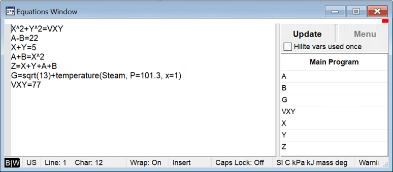
The use of the Computational Flow Window is best illustrated by example. Shown below are set of 7 equations and 7 unknowns.

These equations will solve using the default stopping criteria. It might appear that EES needs to solve all seven equations simultaneously, but this is not the case. EES will automatically identify an efficient way to solve these equations by determining the optimal calculation order, referred to as the blocking. EES first finds constants, such as VXY, and sets their values. Next, it will attempt to solve equations that have a single unknown variable, such as the equation that sets the value of G. The equations in this category are reordered so as to solve as many equations in this way as possible. The order that the equations are solved is shown in the Computational Flow window. Next EES will look for groups of equations that need to be solved simultaneously. In this case, EES identifies that the two equations involving variables X and Y can be solved. The group of equations is referred to as a block. Blocks are numbered sequentially, so this group becomes Block 1. With the values of X and Y now determined, EES can solve the two equations involving variables A and B, which becomes Block 2. Finally, with X, Y, A, and B all known, the value of Z can be found in Block 3.
Select Computation Flow from the Windows menu. By default, the Main program block is selected with blocks shown. Right click on Main to display all of the equations in the Main block. Alternatively, click the + box at the left of each block to display the equations in that block. The + sign will then become a - sign. Click again to hide the equations.
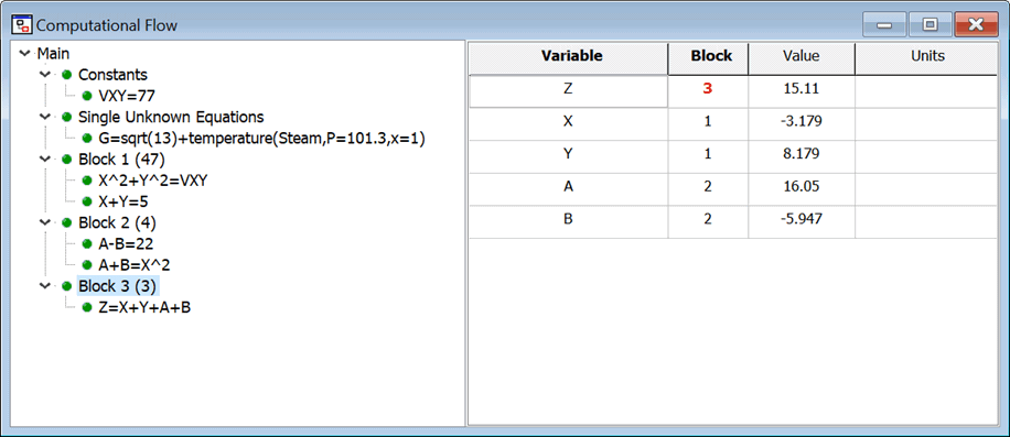
The Computational Flow window is divided into three panes. The pane on the left shows a tree view of all of the blocks involved in the problem. The figure above shows the most common blocks, which include Constants, Single Unknown Equations, and each of the blocks of equations that are solved simultaneously, labeled Block xx, where xx is a number. The parenthesized number that follows the block name is the number of times the block was called during the calculation procedure. Clicking the left mouse button on a block name selects that block. All of the variables that are involved in the equations for the selected block will then be displayed in the top right panel. This panel shows the variable name, the block that its value was determined in, the value of the variable and its units. Variables for which the block number is shown in red have values that are determined in the selected block. For example, the figure above shows the variables involved in Block 3, where the value of variable Z is determined. The variables are initially shown in the order that they appear in the equations for the selected block. Clicking the left mouse button in the Variable cell will reorder the variables so that they are displayed in alphabetical order. Click again to show the variables in reverse alphabetical order. Click a third time to restore the original order. Similar behavior occurs by clicking in the Block cell, which will reorder the list in terms of the block number. Note that the information in the Block column identifies where in the program the variable is defined. If a number is shown, the variable is determined by the equation(s) in the block having this number. However, the block column may display any of the following items.
Const the variable is a constant defined in the Equations window
Single the variable is defined by solving a single equation with it being the only unknown
Integral the variable's value is defined by EES as it is the integration variable in an equation-based integral
Macro the variable is defined in a Macro file or in the Macro Command window
Import the variable is defined by a $Import directive
Table the variable is defined in a Parametric table
MinMax the variable is one of the independent variables set by the MinMax optimization algorithm
Common the variable is defined by a $Common directive
Diagram the variable is defined in the main Diagram Window or in a Child Diagram window
VarInfo the variable is created by EES and used in an equation for guess values or limits in the Variable Information dialog
Input the variable is an input to a Subprogram or Module
Clicking on an equation in the tree view pane will display the variable information for the selected equation, rather than for the selected block. In the display above, block 3 consists of only one equation so the variable display is unchanged. However, a third pane will appear at the bottom right of the window showing the absolute and relative residuals. The absolute residual (Abs. Resid) is the difference between the left and right hand sides of the equation using the calculated values for the variables. The relative residual (Rel. Resid) is the absolute value of absolute residual divided by the value of the left-hand side of the equation, assuming that it is not equal to zero; if the left-hand side of the equation is identically zero, the relative residual will be the same as the absolute residual. During the calculations, a solution is considered to be found if the maximum relative residual value for all equations is less than the Residual Tolerance specified with the Stop Criteria in the Options menu. Also shown in this pane is the number of evaluations (including those required to calculate numerical derivatives) required to solve the equation and the status of the unit checking for the selected equation, the accumulated time in milliseconds needed to solve the equation, and the unit checking status. For unit checking, OK will be displayed if the unit check is successful. A ? will be display if the unit check fails. An X will be displayed if unit checking has been disabled for this equation.
Clicking the right mouse button on an equation in the tree view pane will bring up a popup menu, as shown below.
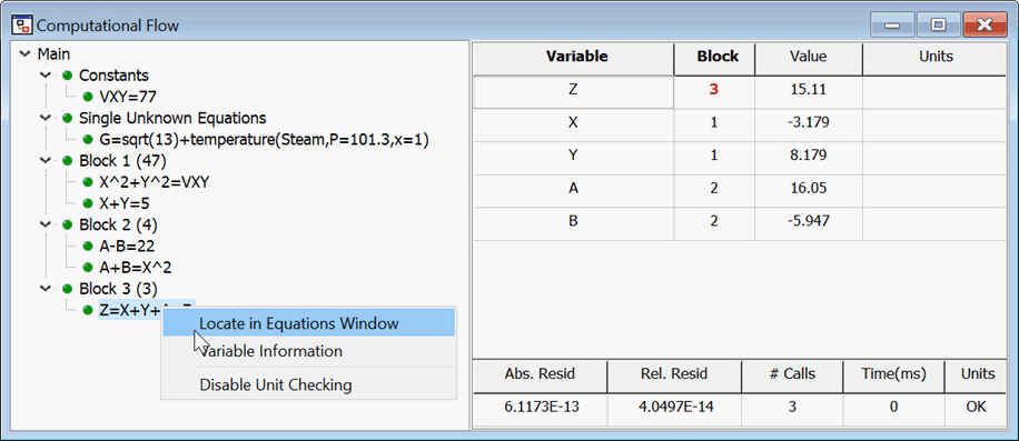
The Locate in Equations Window menu item will bring the Equations window to the front with the selected equation highlighted. The Variable Information menu item will bring up an abbreviated Variable Information dialog showing just the variables in the selected equation where the guess values, limits, and units of the variables can be changed. The Disable/Enable Unit Checking menu item will either disable or enable the unit checking for the selected equation. (It is sometimes convenient to disable unit checking for empirical equations that involve constants with units.)
Clicking the right-mouse button on a variable name or block number in the upper right panel will bring up a pop-up menu with the options shown below.
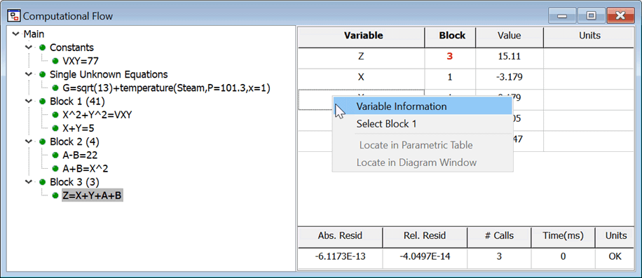
Variable Information displays an abbreviated Variable Information dialog showing just the variables for the selected block or equation. Select Block xx will move the focus of the tree view to the block in which the variable that was selected was defined. The variable display will be changed to show the information for this block. The last two menu items are only enabled if the selected variable was defined in a Parametric Table or in the Diagram window, respectively. In this case, selecting the menu item opens the Parametric table or Diagram window and highlights the column or location where the variable is defined.
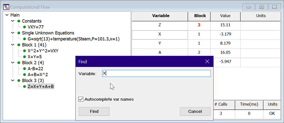
The Find command can be used to show which blocks a variable is defined in. Select Find from the Search menu and enter the name of the variable. Click the Find Next button and the block that contains this variable will be selected showing the equations and variables that use the variable. Click the Find Next button again to move to the next occurrence of the variable.
If EES is configured to manipulate complex numbers, two equations, one each for the real and imaginary parts, will be generated for each equation entered in the Equations window. The real and imaginary equations are identified with a (r) and (i) just to the left of the equation.
The Computational Flow window can be very helpful for identifying the source of conversion problems. As an example, change the value of VXY from 77 to -77 and Solve the equation set. A solution cannot be obtained (unless EES is configured in Complex number mode) and you will see the following error message

Click the Yes button to display the Computational Flow window. Note the small icons to the left of each branch of the tree.
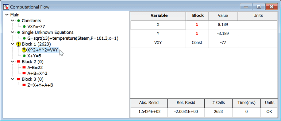
The meaning of these icons is as follows:
![]() Indicates that the equation or block was solved properly
Indicates that the equation or block was solved properly
![]() Indicates that there was a problem solving the equation or the block and it did not solve the desired accuracy
Indicates that there was a problem solving the equation or the block and it did not solve the desired accuracy
![]() Indicates that EES did not need to solve the equation or block because the values were already known. This situation typically occurs when calling a Procedure with multiple outputs.
Indicates that EES did not need to solve the equation or block because the values were already known. This situation typically occurs when calling a Procedure with multiple outputs.
![]() Indicates that EES did not attempt to solve the equation or block due to errors that occurred previous to this point
Indicates that EES did not attempt to solve the equation or block due to errors that occurred previous to this point
![]() Indicates that there appears to be a problem, perhaps a missing equation, that occurs within or before this block.
Indicates that there appears to be a problem, perhaps a missing equation, that occurs within or before this block.
EES was able to exactly locate the problem in this case. In more complicated cases, EES will identify the block, but perhaps not the equation that is causing the convergence problem.
It is possible to display the Computational Flow window in a debugging situation. If the number of equations is less than the number of unknowns, EES will not be able to solve the equation set, but the Computation Flow Window can be made visible by selecting it from the Windows menu. Look for a block preceded by the yellow question mark icon as this likely identifies the location of the missing equation.